Microsoft Excel is one of the best software for small-scale businesses if used to its full capability, but if used incorrectly, instead of making the project easier, it can linger on unnecessarily.
Fortunately, there are ways to make your Excel use more efficient by using some of the software’s secret gems:
1. Flash Fill
Flash fill is an amazing feature that recognizes your data filling patterns and automatically fills the data for you making your work easier. It gets more accurate with time as it learns your typing patterns.
- Combining texts in 2 different tabs, e.g., Combing first name and last name
- Extracting text from, say given tab, e.g., extracting user-ids from email addresses
- Formatting phone numbers and email addresses
To use this feature:
- Go to Data > Flash Fill to run it manually, or press CTRL + E.
- To turn Flash, fill on, go to Tools > Options > Advanced > Editing Options > check the Automatically Flash Fill box.
2. Watch Window
Excel’s watch window is the best tool to double-check your formulas and calculations. It is a floating window that lets you view the content of any tab not visible on the screen making it convenient to inspect, audit, or confirm formula calculations and results in large worksheets without scrolling around.
To use this feature:
- Select the cells that you want to watch.
- On the Formulastab, in the Formula Auditing group, click Watch Window.
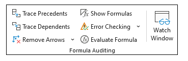
- Click Add Watch, and you are done.
3. Conditional Formatting
Conditional Formatting in Excel is one such feature that is present right under the user’s eyes on the home tab. This editing and highlighting feature is often overlooked by beginners. Conditional formatting offers a vast range of customizations based on cell data.
To use this feature:
- Select the range of cells, the table, or the sheet for which you want to apply conditional formatting.

- On the Hometab, click Conditional Formatting.
- Choose from the various options available.
4. Paste Special
Sometimes you wish to copy certain parts of a cell like their formulas, typeface, color, and font size and not the content. This paste special option does exactly that by maintaining the original formatting or copying it and pasting it on other cells.
For e.g., using the formulas option under the paste special window, you can paste the formula of a specific cell on another cell.
To use this feature:
- Cut or copy the picture, text, or object that you want to paste.
- Click on the place you wish to insert that item.
- On the Hometab, in the Clipboard group, click the arrow under Paste, click Paste Special, and then choose one of the options given.
5. Sparklines
Excel is a user-friendly software with easy to navigate interface, graphs and visuals are a great way to represent data, but things can get a bit messy when graphs are mixed with data.
Sparklines solve this issue by adding small charts to various cells’ backgrounds. These make it easier to observe patterns while quickly glancing over spreadsheets. A sparkline is a tiny chart in a worksheet cell that provides a visual representation of data.
Use sparklines to show trends in a series of values, such as seasonal increases or decreases, economic cycles, or to highlight maximum and minimum values. Position a sparkline near its data for the greatest impact.
To use this feature:
- Select a blank cell at the end of a row of data.
- Select Insert and pick Sparkline types, like Line or Column.
- Select cells in the row and hit
- More rows of data? Drag the handle to add a Sparkline for each row.
- Finally, format the sparkline to select the type of in-line chart, and you are good to go.
6. Power View
Power View is a data visualization technology that lets you create interactive charts, graphs, maps, and other visuals that bring your data to life.
Power View is available as an add-in for Excel. Once the power view is added the power view tab is available.
The different Power View visualizations that you can have are as under:
- Table
- Matrix
- Card
- Charts
- Line Chart
- Bar Chart
- Column Chart
- Scatter Chart
- Bubble Chart
- Map
7. Pivot Tables
A Pivot Table is a powerful tool to calculate, summarize, and analyze data that lets you see comparisons, patterns, and trends in your data.
Without having to look through the whole spreadsheet, it will help you regroup your data from different perspectives.
You can get a better understanding of your data. PivotTables work a little bit differently depending on what platform you are using to run Excel.
To use this feature:
- Select the cells you want to create a Pivot Table from.
- Navigate to Insert> PivotTable
- This will create a Pivot Table based on an existing table or range.
- Click OK, and you are ready to unleash the power of pivot tables.
We hope you enjoyed this article about the 7 amazing excel features. Try to master these hidden gems, and you will become an Excel Ninja in no time.